I found it pretty hard to understand im2col at first, so just gonna dump my thought process here.

IM2COL Motivation

Convolution is naturally written as a sliding-window operation: for every output position, we collect a small neighborhood from the input and take an inner product with the kernel. That description is intuitive, but it is not always the most convenient shape for modern accelerators. GPUs are extremely good at dense matrix multiplication, especially when the work can be expressed as large GEMMs that map cleanly onto tensor cores. A naive convolution loop, on the other hand, usually exposes the computation as many tiny dot products with complicated indexing.

IM2COL is a way to bridge that gap. Instead of thinking of convolution as “move the kernel across the input”, we materialize, or logically view, each sliding window as a row in a matrix. The kernel is flattened into another matrix. Once both sides are arranged this way, the convolution becomes a GEMM:

This transformation does not change the math. It changes the layout of the work. That layout matters because a GEMM gives the compiler and hardware a much clearer structure: contiguous tiles, predictable memory movement, shared-memory reuse, and tensor-core friendly matrix fragments. Even when the full im2col matrix is not explicitly written to global memory, the same idea is often used inside a tiled kernel: stage a local patch of the input, reshape it into the matrix shape expected by GEMM, multiply, and reshape the result back.

The tradeoff is that im2col can duplicate input elements. Neighboring sliding windows overlap, so the same input value may appear in multiple rows of the lowered matrix. In a literal implementation, that costs extra memory bandwidth and storage. In optimized kernels, the trick is to do the lowering inside a tile or in shared memory so we get the GEMM-friendly compute structure without paying the full global-memory cost.

IM2COL

In tilelang the im2col is extremly simple:

@tilelang.jit(
    pass_configs={
        tilelang.PassConfigKey.TL_DISABLE_WARP_SPECIALIZED: True,
        tilelang.PassConfigKey.TL_DISABLE_TMA_LOWER: True,
    },
)
def tl_conv1d_im2col(X, K, BLOCK_N: int, BLOCK_L: int):
    N, L, KL, F = T.const("N, L, KL, F")
    dtype = T.float16
    accum_dtype = T.float32
    X: T.Tensor((N, L), dtype)
    K: T.Tensor((KL, F), dtype)
    O = T.empty((N, L, F), dtype)

    with T.Kernel(N // BLOCK_N, L // BLOCK_L, threads=256) as (pid_n, pid_l):
        X_shared = T.alloc_shared((BLOCK_N, BLOCK_L, KL), dtype)
        K_shared = T.alloc_shared((KL, F), dtype)
        O_local = T.alloc_fragment((BLOCK_N * BLOCK_L, F), accum_dtype)

        for i, j, k in T.Parallel(BLOCK_N, BLOCK_L, KL):
            X_shared[i, j, k] = T.if_then_else(
                pid_l * BLOCK_L + j + k < L, X[pid_n * BLOCK_N + i, pid_l * BLOCK_L + j + k], 0
            )
        X_reshaped = T.reshape(X_shared, (BLOCK_N * BLOCK_L, KL))
        T.copy(K, K_shared)
        T.gemm(X_reshaped, K_shared, O_local, clear_accum=True)
        O_reshaped = T.reshape(O_local, (BLOCK_N, BLOCK_L, F))
        T.copy(O_reshaped, O[pid_n * BLOCK_N, pid_l * BLOCK_L, 0])
    return O

Basically we do

1. Flatten X
2. Reshape X
3. GEMM
4. Reshape back O
5. Write back

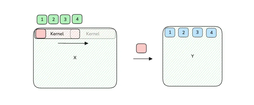
In the above minimal example, the input X has shape (N, L) and the kernel K has shape (KL, F). Since F is the channel dimension, we can don’t care too much about it since it can be broadcasted across X (in simpler words, whatever arithmetic you do to X in F=1 case, just do it again using the value on kernel for F=2). So, we can just see it as a 1d convolution across the L dimension on X.

In order to compute the convlution, an intuitive way is to think of this as sweeping the kernel across the input. The output element is computed by $O_{i,j} = \sum_{m=0}^{KL} X_{i, j+m} \cdot K_{m}$. Notice that it’s similar to the inner product of two vectors.

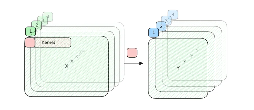
The key here is to think of the action of “sweeping” as extending to a third dimension, and each layer in that dimension exactly captures a snapshot of the matrix that the kernel see at that moment. For example, if kernel has length of 4, then in the “sweeping” view, when $t=0$, the kernel is aligned to the first element, so it sees 1st, 2nd, 3rd, 4th (i know i should use 0-index here, but i don’t want to redraw the figure). When $t=1$, the kernel sees 2nd, 3rd, 4th, 5th. So for the first matrix position, in timestamp 1, 2, 3, …, the kernel sees 1st, 2nd, 3rd, … element as well. If we extend that to an extra dimension, we are able to layout the entire sweeping process to be a big matrices of snapshots.

If we reshape the extended matrix to only the inner dimensions, we can see clearly how it is equivalent to matmul.

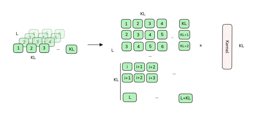Since it’s tiled, the case for an inner tile is different from a tail tile. For the inner tile, we don’t need to deliberatly boundary check anything, because the kernel can sweep across every single element in the tile. For tail tile, we need to make sure that the kernel is not sweeping outside the input, so we need boundary check and mask them.

In the figure above, you can see the element index can actually go beyond L. This is because the L here, in the context of a tile, is actually BLOCK_L. The element outside this tile also contribute the output for this tiles.

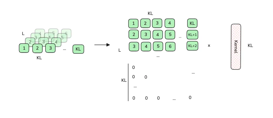
However, if we reaches for example the last block, we need to set those indexes beyond L to be 0 because they are truly out of bound.